Innovations In Cement Manufacturing: Complete Guide & Downlo

Innovations in Cement Manufacturing Chapter 10.2, Modeling in Cement Kiln Operations, is the section of the Portland Cement Association’s master reference that explains how mathematical modeling transformed the understanding and the operation of the clinker-burning line. The rotary kiln is a hostile environment, impossible to instrument completely inside and too slow and too expensive to experiment on by trial and error, so the industry learned to represent it on paper and in code: models that compute the heat and mass flows, the temperatures along the kiln, the flame and the combustion, the charge and the refractory, the kiln rotation and the gas flow, and the dynamic response of the whole system to the changes of the feed and the fuel. This guide develops Chapter 10.2 for the modern engineer: the physical foundations of the kiln, the families of models (steady-state balances, empirical statistical models, one-dimensional kiln models, computational fluid dynamics and dynamic simulators), the discipline of calibration and validation with the plant data, and the applications that made the modeling the daily instrument of the operation, the optimization, the design and the training of the cement industry. The chapter is read here not as a history but as the intellectual toolbox that every modern plant still uses, now amplified by the digital twins of our decade.

1. Why the Kiln Had to Be Modeled

The rotary kiln resists every direct approach of the experimenter. Its interior temperatures reach 1450 °C in the material and 1800 °C in the flame; its length often exceeds 60 metres (up to 120 metres in the old wet and long dry kilns); its charge tumbles and cascades, its gas flows counter-current; its residence time runs to tens of minutes or hours; and the internal reactions, the calcination, the melt formation and the clinkering, are tightly coupled to the heat transfer. One cannot cheaply instrument the interior, scale down the process without changing the physics, or pause the operation to take a measurement. The result of more than a century of this difficulty is that the quantitative understanding of the kiln was built primarily through models: first the hand-calculated balances of the pioneer engineers, then the desk computers of the 1960s and 1970s, and now the high-resolution simulations of the modern workstations. Modeling was not an option for the industry; it was the only route to quantitative reasoning about the heart of the process.

The consequences of this modeling history are visible in every modern plant. The preheater tower, the precalciner, the burner design and the refractory profile were all developed and optimised with the support of models before they were installed. The operating procedures (the fuel split, the excess air, the kiln speed, the turning and the burning-zone control) are today derived from the models, and the operator’s display is a live, simplified model of the line. The modern “digital twin”, in which the model of the plant runs parallel to the real plant, is nothing but the latest and most complete form of this century-long modeling project, which is why Chapter 10.2 remains a foundational reading for the process engineer, the control engineer and the design engineer alike.

2. The Physical Foundations: The Physics the Models Must Reproduce

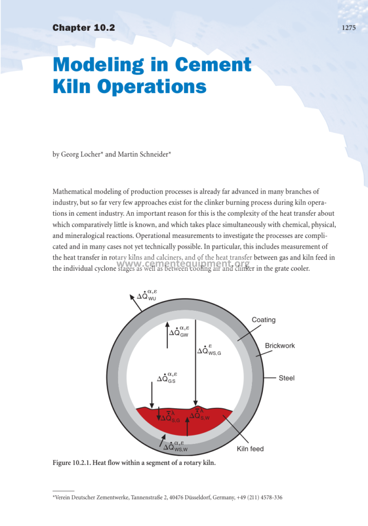
Every kiln model, however sophisticated, rests on the same physical foundations, and the modeller who does not respect them produces untrustworthy numbers. The first foundation is the heat transfer, for which the kiln is a complex network: radiation from the flame and the hot gas to the exposed charge and the refractory; radiation from the refractory to the charge; conduction through the charge and the refractory; convection in the gas; and the rotation that periodically exposes the material to the flame and then buries it under a new crescent ^{of material}. The second foundation is chemical kinetics: the drying, the volatiles, the calcination of the carbonates (a strongly endothermic decomposition with its temperature and CO₂ dependence), the melt formation and the clinkering, each with its own rate. The third is transport phenomena: the axial movement of the charge (a function of the kiln slope, the rotation speed, the filling and the material properties), the gas flow and the mixing, the residence-time distribution of the solids and the gases. The fourth is the thermochemistry: the heat of formation of the clinker, the specific heats, the enthalpies of the reactions and of the raw materials as the composition changes along the kiln.

The models differ in how completely they couple these foundations. The steady-state axial models solve the one-dimensional energy and mass balances along the kiln axis; the zonal models divide the kiln into a few well-mixed zones (the preheat zone, the calcination zone, the burning zone, the cooling zone) and balance each; the two-dimensional and three-dimensional models, including the computational fluid dynamics of the flame and the charge, resolve the spatial fields. Whatever the level, the modeller’s first duty is the honest statement of the assumptions: the kinetics constants, the heat transfer coefficients, the particle size, the charge motion model and the property correlations, each of which carries its uncertainty, and the hierarchy of the uncertainties must be propagated into the final results. A model is only as good as the honesty of its assumptions and the quality of its validation, and this is the discipline that separates the professional modelling chapter from the calculator exercise.

3. The Steady-State Balance Models: The Foundation of the Audits

The simplest and still the most used models in the industry are the steady-state mass and energy balance models, the same mathematics of the classical heat balance. The inputs are the measured flows: the kiln feed and its composition, the fuel flow and its heating value, the secondary and tertiary air, the kiln exit gas composition, the cooler air and the clinker flow and temperature; the outputs are the estimated heat consumptions, the losses and the efficiencies. The balance is written around each process node (the preheater, the calciner, the kiln, the cooler) and around the whole system, and the closure of the balance verifies the inputs, because a heat balance that does not close to within a few percent reveals an error in the measurements or in the assumptions. These models are the tool of every thermal audit, the comparison of the designed and the actual performance, the fuel and the raw material evaluation, and the investment studies (for example, the benefit of a new preheater stage or a new cooler), and they are fast, transparent and trusted because their mathematics is simple and the data are the real figures of the plant.

Their limitation is precisely their steady-state nature: they describe the mean operating point, not the dynamics, and they cannot reveal the cause of an instability or the path of a transient. This is why the industry built on the balance models with the steady-state axial models on one side (to resolve the internal profiles) and the dynamic models on the other (to study the time-dependent behaviour). The balance model also taught the industry the language of the specific heat, the specific electrical energy and the energy allocation, which is still the language of the modern reporting, and a plant that runs its monthly energy balance with a validated steady-state model has the foundation on which all the other models are calibrated and to which all the optimisations are compared.

4. The One-Dimensional Axial Model: Resolving the Inside of the Kiln

The one-dimensional axial model goes one decisive step beyond the box balance: it discretises the kiln into a series of finite slices along the axis and solves in each slice the balances of the energy of the gas, the energy of the solids and the energy of the wall, coupled by the radiation view factors and the convective heat transfer, together with the kinetics of the calcination and the clinkering and the axial movement of the charge. The output is the axial temperature profile of the gas, the solids and the wall; the progress of the calcination along the kiln; the position and the length of the burning zone; the heat transfer breakdown at each slice; and the overall thermal performance. These models are the standard tool of the kiln design and the retrofit studies: they show where the heat is used and lost, where the calcination finishes, how the flame position and the burner momentum move the profiles, and what the effect of the kiln speed, the fill and the refractory thickness would be.

The calibration of such a model with the plant data is the professional art. The measured boundary values (the inlet and the outlet temperatures, the gas composition, the flame characteristics) fix the consistent solution, and the adjustable parameters (the emissivities, the kinetics pre-factors, the charge-movement factors) are tuned within their physical ranges until the model reproduces the measured axial thermocouples and the kiln exit conditions. The validated model then becomes a virtual laboratory: the engineer can test the effect of a different burner, a higher secondary-air temperature, a lower excess air, a different kiln speed, without touching the real kiln, and the ranking of the options from the model is then confirmed by the plant trials. This use of the axial model, as the virtual experimenter of the burning line, is exactly what Chapter 10.2 celebrates as the innovation of the modeling approach.

5. Empirical and Statistical Models: Learning from the Data

Parallel to the physical models, the industry developed the empirical and the statistical models, which learn the behaviour of the kiln from its operating data rather than from the first principles. The regression models correlate the dependent variables (the burning-zone temperature, the free lime, the heat consumption) with the measured factors (the feed, the fuel rate, the oxygen, the kiln speed), and their coefficients are estimated from the historical data; they are quick to build and easy to use in the control logic, but they retain their validity only within the range of the data on which they were fitted, so they must be re-fitted when the operating point changes. The grey-box models combine the physical structure of a balance with the empirical estimation of the unknown parameters, giving the physical insight plus the data-driven calibration, and they are the compromise most used in the practice.

The modern form of the statistical modelling is the use of the artificial neural networks and the machine learning: the network is trained on the collected data of the plant to map the inputs to the outputs, with the hidden layers capturing the nonlinear couplings that the analytical regression cannot. The neural models proved particularly useful for the prediction of the free lime and the clinker quality from the process variables, for the fault detection (the networks that recognise the abnormal patterns as early as the data allow), and as the internal models of the advanced controllers. The chapter’s hypothesis of 2004 has been fully realised in the data-rich plants of today, where the historian and the machine learning operate side by side, but the professional caution remains the same: the data models must be validated on the independent data, monitored for the drift, and never extrapolated blindly outside the trained envelope, because a statistical model that has never seen a condition cannot know its answer.

6. Computational Fluid Dynamics: The Flame and the Gas Field

The highest-fidelity models resolve the three-dimensional fields of the kiln interior with the computational fluid dynamics (CFD): the turbulence, the radiation, the combustion chemistry and the particle transport of the burner flame and the gas flow, and, in the advanced codes, the granular flow and the heat transfer of the charge. The CFD model of the burner and the burning zone is the instrument with which the modern burner designs, the flame shapes and the momentum and the swirl settings are optimised, and it answers the questions that the axial model cannot: the recirculation zones, the oxygen distribution near the flame, the temperature field of the gas that the axial model averages, the CO and the NOx formation, and the interaction of the flame with the charge in the burning zone. The CFD is also used on the preheater cyclones (the separation efficiency, the pressure drop, the erosion), on the calciner vessels (the suspension, the burnout of the fuel) and on the cooler (the air distribution and the heat recovery).

The cost of the CFD is high: the meshing, the physics, the turbulence models and the computational time demand the specialist, and a full three-dimensional kiln case can run for days even on the modern processors, which is why the industry uses CFD as the deep-analysis tool on the critical problems, reserving the faster models for the routine. The validation of a CFD result with the plant data is indirect (the interior is not instrumented), so the professional uses the global measurements (the exit gas, the shell scanner, the clinker temperatures) and the proven sub-models to gain confidence, and he treats the CFD as the source of qualitative insight and design direction rather than the absolute truth. The chapter’s view of the modeling hierarchy, from the balance to the CFD, remains the exact framework that the modern kiln-modelling community applies, and the CFD is the frontier where the modeling of the flame meets the reality of the fuel and the alternative fuels of today.

7. Dynamic Models and Simulators: The Time Dimension

The dynamic models add the time, and with it the possibility of studying the transients, the stability and the control, which are the operational realities of the kiln. The dynamic model of the kiln system descends from the state of the steady-state model: the energy and the mass balances become differential equations with the residence times, the transport lags and the thermal inertias of the refractory and the charge, and the model responds to the changes of the feed, the fuel and the draught with the same lags and the same dynamics as the real line. Such a model is the foundation of the operator training simulator, in which the trainee operates a virtual kiln that behaves realistically, and it is the laboratory of the control design: the advanced controllers and the tuning strategies are first tested on the model before they are applied to the plant. The dynamic model also reveals the stability limits of the operation: the point at which a small perturbation develops into an oscillation, the effect of the delays on the controllability, and the design of the feedforward compensation that the plant cannot avoid because of the long dead time.

The fidelity of a dynamic model is limited by the fidelity of its thermal and chemical dynamics, and the most demanding part is the representation of the charge motion and the melt, which changes the heat transfer with the temperature and the composition. The industry therefore uses the dynamic models at the appropriate level: the simplified dynamic balances for the control and the training, and the more complete versions for the dedicated studies, always calibrated against the step tests and the historical transients of the plant. The value of the dynamic approach is proven by the modern trend of the digital twin: a live, continuously updated dynamic model of the plant that runs in parallel with the operation, used for the prediction, the optimisation and the operator decision support, which is the latest and most complete realisation of the modeling programme that the chapter of the PCA volume inaugurated.

8. Modeling the Complete Plant: From the Quarry to the Finish Mill

The final step of the modeling ambition is not the kiln alone but the complete plant, which the chapter and the modern software address with the flowsheeting approach: a single model that represents the crusher, the raw mill, the homogenisation, the preheater, the calciner, the kiln, the cooler, the finish mill and the storage, connected by the material and the energy streams. The plant model computes the specific energies, the mass balances, the emissions and the end-to-end behaviour, and it answers the questions that cross the process boundaries: the effect of the raw-material variability on the whole line, the optimal operating point of the mill versus the kiln, the allocation of the electrical and the thermal energy through the plant, and the sensitivity of the production to each bottleneck. The plant model is the instrument of the design of the new installations (the new line is simulated before the construction), of the debottlenecking studies of the existing plants, and of the benchmarking that compares the sections of the plant against the reference designs.

The modern flowsheeting of the cement plant is aided by the graphical simulation environments, in which the engineer builds the model on the screen with the components and the property packages, and the solver converges the complete set of the balances. The integration with the cost models and the life-cycle tools extends the flowsheeting into the economics: the model can compute the cost per tonne as a function of the fuels, the additions, the electricity and the market, which transforms the flowsheeting from an engineering instrument into a decision instrument. For the operator of a single plant the complete-plant model is the tool of the daily optimisation; for the group it is the instrument of the benchmarking between the plants, the sharing of the best practice and the planning of the capital; and the power of this approach, already visible in the chapter, is now magnified by the continuous real-time data of the digital twin.

9. Modeling the Challenges of the Modern Kiln: Alternative Fuels, Emissions and the Energy Transition

The modeling of the kiln did not stop at the classical coal-fired operation; it became the essential instrument of the modern challenges, and the first of them is the alternative fuels. A waste-derived fuel burned in the calciner or at the kiln inlet brings a heterogeneous particle, a variable heating value, a higher moisture and a different chemistry, and the physical models are the only way to predict the effect before the fuel is accepted: the axial model computes the extent of the burnout and the temperature profile with the coarse solid particles, the CFD resolves the mixing and the combustion of the multi-size fuel in the burner and the calciner, the dynamic model calibrates the stability margin when the feed of the fuel fluctuates, and the balance model computes the ash input and the raw-mix correction that the new fuel demands. The result is that the modern plants use the models to evaluate, accept and plan the fuel portfolio, increasing the substitution rate with confidence and minimising the process risk, exactly the application that the chapter of 2004 anticipated and that the energy transition has made central.

The models serve the emissions targets with equal power. The NOx formation in the flame depends on the temperature and the oxygen fields that the CFD resolves, and the models are used to design the staged combustion, the SNCR injection of the reductant and the oxygen profiles that reduce NOx without increasing CO; the SO₂ and the volatile cycles (sulfur, alkali, chloride) are modelled as the circulation rates that decide the bypass need; the CO₂ of the process is computed from the flowsheet balances that allocate it to the clinker, and the carbon-lean and hydrogen-blended future fuels are being studied in the models before they touch the commercial lines. The energy transition, the electrification and the carbon capture are likewise model-intensive designs: the oxy-fuel kiln with its CO₂-rich gas, the calciners with the captured CO₂, and the electrified alternatives are all being developed first in the simulated kilns. The modeling that began as the way to understand the classical burning line has become the universal laboratory of every future kiln, and the chapter’s method, the disciplined representation of the physics with the validated data, is exactly the method with which the industry will design the cement plants of the decarbonised era.

10. Calibration, Validation and the Honest Use of the Numbers

Whatever the type of model, its professional value is decided by the calibration and the validation, and the chapter’s implicit lesson is that the model is a living tool, not a published document. The calibration fixes the free parameters (the emissivities, the kinetics, the heat-transfer coefficients, the statistical coefficients) against the measured behaviour: the steady-state against the measured balances and the axial profiles, the statistical against the historical data, the dynamic against the step tests and the transients. The validation then tests the calibrated model on the independent data that were not used in the calibration, the true test of the generalisation, and the model that fails the validation is corrected or rejected. The documentation of the assumptions, the data, the fits and the residuals is the professional evidence, and the version control of the models accompanies the version control of the plant, because a model calibrated for one burner or one fuel is not automatically valid for another.

The honest use of the numbers is the final discipline. The engineer communicates the results with their uncertainty, distinguishes the well-validated predictions from the extrapolations, and never lets the model replace the engineering judgement of the plant reality. The industry has learned this lesson the hard way: the models have been wrong when the physics was mis-specified, when the data were biased, or when the operating range was left, and the memory of those errors is precisely what makes the modern profession insist on the validation. The balanced view, which the chapter teaches, is that the model is neither infallible nor useless: it is a quantified, disciplined, constantly corrected representation of the plant, and used with that honesty it multiplies the engineer’s power, which is why the modeling is today as standard in the kiln department as the calculator in the office.

11. Applications: Design, Optimisation, Operation and Training

The four great applications of the kiln modeling, which the chapter organises implicitly in its structure, are:

Application	Model used	Result achieved
Design of new lines	Plant flowsheet + axial kiln + CFD	Size, energy, emission and cost prediction before construction
Retrofit and debottlenecking	Axial kiln, cooler and plant models	Ranked options with the energy and production benefits
Daily optimization	Steady-state balances + statistical models	Best operating point for the given market and fuels
Advanced control and stability	Dynamic models, neural and MPC	Stable burning zone, reduced variability and heat
Operator training	Dynamic simulators	Practice of the start-ups, upsets and emergencies
Digital twin and prediction	Live dynamic plant model	Prediction, decision support and anomaly detection

In the design, the model replaces the expensive trial on real installations; in the optimisation, it finds the operating point that the experiments on the live plant could never explore; in the control, it provides the structure and the tuning of the advanced systems that now run the burning zone; in the training, it gives the operators the safe rehearsal of every scenario; and in the digital twin, it runs the plant’s twin in real time for the prediction and the decision support. The application that a plant chooses depends on its needs and its people, but the underlying capability, the quantified representation of the kiln, is the same, and the plant that builds it once creates the permanent instrument of its process intelligence.

12. Frequently Asked Questions

Why is the kiln modelled instead of measured directly?

Because the interior at 1450 °C cannot be fully instrumented, the process cannot be scaled down without changing the physics, and the trial-and-error experiments are too expensive and too slow; the model is the only practical way to reason quantitatively about the inside of the kiln.

What is the difference between a steady-state and a dynamic model?

A steady-state model describes the mean operating point (the mass and energy balances, the axial profiles); a dynamic model includes the time, the lags and the inertias, so it can simulate the transients, the stability and the control and serve as the training simulator.

Is a neural network model trustworthy for the kiln?

It is trustworthy only within the envelope of the data on which it was trained and only after the validation on the independent data; its advantage is the capture of the nonlinear couplings, and its risk is the extrapolation beyond the experience, so it is used with the physical models as its guard.

How is a kiln model validated with the plant data?

By calibrating the free parameters against the measured balances and profiles, then testing the calibrated model on the independent data; the closure of the heat balance and the agreement of the predicted axial temperatures with the measured ones are the principle checks.

What is the digital twin of the kiln?

It is a live dynamic model of the plant that runs in parallel with the real operation, continuously updated with the real data, and used for the prediction, the optimisation, the anomaly detection and the decision support, the modern realisation of the modelling approach of the chapter.

Do the models also cover the preheater, the calciner and the cooler?

Yes: the same families of models are used on the whole pyro line, the CFD on the cyclones and the calciner, the balance and the axial models on every vessel, and the complete-plant flowsheet connects them all into a single representation.

Is modeling a design tool or an operation tool?

Both: it is a design tool when a new line or a retrofit is studied, and an operation tool when the daily balances, the optimisation, the control and the training run on the models; the same physics and the same validation discipline serve both lives.

13. Summary and Conclusion

Modeling in cement kiln operations is the intellectual core of the modern burning line: the family of quantitative representations, from the hand-written heat balance to the CFD of the flame and the live digital twin, that replaced the guesswork and the trial and error with the disciplined estimation of the design, the optimisation, the control and the training. The physics of the heat transfer, the kinetics and the transport is the common foundation; the steady-state balances, the axial models, the empirical and the neural models, the CFD, the dynamic simulators and the complete-plant flowsheets are the successive levels of the ambition; and the calibration, the validation and the honest use of the numbers are the professional discipline without which the models deceive. The chapter of the PCA volume documents the birth of this programme, and the industry of today runs on its continuation: the same models, now fed by the continuous data of the DCS and the historian, running as the virtual laboratories and the digital twins of the plants. The engineer who has mastered the modeling of the kiln holds the instrument that every design decision, every optimisation campaign, every operator formation and every digital transformation of the industry depends on, and that competency, exactly as the chapter teaches, is the competency of the modern cement process analyst.

This file is part of the Complete Cement Technical Package (931 files) available from cementequipment.org. Respective rights holders; library copy for the licensed single user.